Image Recognition in Julia using Flux
In this short post, we will learn a simple character recognition model in Julia using the Flux package step-by-step. I’ll be introducing:
- Loading CSV data.
- Splitting data.
- Using Flux.DataLoader.
- Writing a model in Flux.
- Training a model in Flux. (Using the GPU)
- Logging error during training.
The dataset we’ll be using is the Arabic Character Dataset on Kaggle.
Loading CSV files:
Before doing anything, make sure the csv files are unpacked from the archive.
In order to load the CSV files, we’ll need two packages, CSV and DataFrames. CSV is for reading the CSV file itself, and DataFrames is for formatting the output of the CSV.read stream.
using csv
using DataFrames
Next we’ll get our input.
train_data_input = CSV.read("csvTrainImages 13440x1024.csv", DataFrame)
test_data_input = CSV.read("csvTestImages 3360x1024.csv", DataFrame)

train_label_input = CSV.read("csvTrainLabel 13440x1.csv", DataFrame)
test_label_input = CSV.read("csvTestLabel 3360x1.csv", DataFrame)
In case you’re running this in Jupyter I highly recommend putting this bloc in its own cell to avoid running it more than once. Especially when working in Colab where disk operations take some time.
Data processing and DataLoader:
During data processing we’ll need 4 more functions, 2 from MLDataPattern and the last two from Flux:
using MLDataPattern:shuffleobs,splitobs
using Flux: onehotbatch, DataLoader
train_data = reshape(Array(train_data_input),:,32,32)/255;
test_data = reshape(Array(test_data_input),:,32,32)/255;
train_data = reverse(train_data,dims=(2));
test_data = reverse(test_data,dims=(2));
train_label = reshape(onehotbatch(Array(train_label_input),1:28),28,13439);
test_label = reshape(onehotbatch(Array(test_label_input),1:28),28,3359);
train_data = permutedims(train_data,[2,3,1])
train_data = reshape(train_data,32,32,1,13439)
test_data = permutedims(test_data,[2,3,1])
test_data = reshape(test_data,32,32,1,3359)The first 2 lines are for loading the DataFrame objects we get from reading the csv files.
Next, I had to reverse the 2nd dimension since it came the wrong way around for the heatmap function. It doesn’t matter for the neural network, but it makes visualization easier.
In the next 2 lines, we process the label files. First we use onehotbatch to get the one hot array, with 1:28 because there are 28 characters in the Arabic alphabet. The output of the function is a 28×3359×1 Array. We thus reshape it to our desired size.
We then permute the dimensions in the data arrays to make sure we get what we want after reshaping, then we reshape to 32x32x1x13439. Flux requires the arrays to be in WHCN format (Width-Height-Channel-N), we have 1 channel in our case.
(data,label) = shuffleobs((train_data,train_label))In this line we shuffle the training data for partitioning. This is important as the dataset is ordered alphabetically.
(train_data,train_label), (val_data,val_label) = splitobs((data,label), at = 0.85)This line is straight forward. It cuts the training data into a training dataset and a validation dataset at 0.85. So 15% of our data goes to validation and the rest to training.
train_loader = Flux.DataLoader((data=Float64.(train_data),label=Float64.(train_label)),batchsize=128,shuffle=true)
val_loader = Flux.DataLoader((data=Float64.(val_data),label=Float64.(val_label)),batchsize=128)Here we use the DataLoader function from Flux to cut the data into mini-batches. The syntax of DataLoader has changed over time and now it takes the data and the labels in the form of a named tuple. We also shuffle the training dataset for good measure. Cutting the validation dataset into mini-batches eases calculating the validation loss on the GPU later on.
We can wrap this up nicely into one function:
function get_data()
train_data = reshape(Array(train_data_input),:,32,32)/255;
test_data = reshape(Array(test_data_input),:,32,32)/255;
train_data = reverse(train_data,dims=(2));
test_data = reverse(test_data,dims=(2));

train_label = reshape(onehotbatch(Array(train_label_input),1:28),28,13439);
test_label = reshape(onehotbatch(Array(test_label_input),1:28),28,3359);

train_data = permutedims(train_data,[2,3,1])
train_data = reshape(train_data,32,32,1,13439)

test_data = permutedims(test_data,[2,3,1])
test_data = reshape(test_data,32,32,1,3359)
#Validation
(data,label) = shuffleobs((train_data,train_label))
(train_data,train_label), (val_data,val_label) = splitobs((data,label), at = 0.85)
train_loader = Flux.DataLoader((data=Float64.(train_data),label=Float64.(train_label)),batchsize=128,shuffle=true)
val_loader = Flux.DataLoader((data=Float64.(val_data),label=Float64.(val_label)),batchsize=128)
return train_loader, test_data, test_label, val_loader
endThe model:
function network()
  return Chain(

    Conv((3, 3), 1=>16, pad=(1,1), relu),
    x -> maxpool(x, (2,2)), #16x16
    BatchNorm(16),

    Conv((3, 3), 16=>32, pad=(1,1), relu),
    x -> maxpool(x, (2,2)), #8x8
    BatchNorm(32),


    Conv((3, 3), 32=>64, pad=(1,1), relu),
    x -> maxpool(x, (2,2)), # 4x4
    BatchNorm(64),

    Flux.flatten,
    Dense(1024,256), #4x4x64 = 1024
    Dropout(0.2),
    Dense(256,28),

    softmax,)
end
I define here 3 convolutional layers with maxpool and batch normalization to speed up learning. The kernel size chosen is 3x3 since it should give good performance at this input array size. All while keeping in mind the output array size from the maxpool layers.
Next, we flatten the array to go to the Dense layers. I chose to use 2 dense layers with a dropout in-between to reduce overfitting. The final layer should have 28 output neurons for the 28 characters. Then we end with a softmax since this is a classifier.
Training the model:
We’ll need Flux at this point
using Fluxmodel = network()
model = gpu(model)The second line is to offload the model to the GPU for training.
loss(x,y) = crossentropy(model(x),y)
ps = params(model)
opt = ADAM(0.0005)We define the loss function, cross-entropy (Or categorical cross-entropy in TensorFlow terms), as well as the optimizer ADAM at learning rate 0.0005. We’ll also need to define the parameters of the model for training. We’ll only need to define this once.
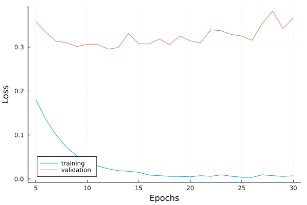
val_error = zeros(epochs)
train_error = zeros(epochs)
val_error_current = 0.
train_error_current = 0.We’ll be using these to track the progress of the error throughout training.
for epoch in 1:epochs
for (x,y) in train_loader
x = gpu(x)
y = gpu(y)
gs = Flux.gradient(() -> loss(x,y),ps) # Gradient with respect to ps
train_error_current += loss(x,y)
Flux.update!(opt,ps,gs)
end
for (x,y) in val_loader
x = gpu(x)
y = gpu(y)
val_error_current += loss(x,y)
endIn order to train, we go through each (data,label) mini-batch in the train_loader (Line 2), we offload the pair to the GPU then calculate the gradient of the loss function with respect to ps. We then calculate the loss for the mini-batch and update the parameters based on the gradient.
For validation, we go through each mini-batch again while only calculating the gradient.
train_error_current /= length(train_loader)
val_error_current /= length(val_loader)
val_error[epoch] = val_error_current
train_error[epoch] = train_error_current
println("Epoch: ", epoch)
println("Validation error: ", val_error_current)
println("Training error: ", train_error_current)
println("===========================")
val_error_current = 0.
train_error_current = 0.Next we divide the errors by the number of mini-batches and update the error vectors. As a bonus, I also make it output a message at each epoch due to impatience.
We can wrap this up in a function again:
function train_model(epochs)
model = network()
model = gpu(model)
loss(x,y) = crossentropy(model(x),y)
ps = params(model)
opt = ADAM(0.0005)
val_error = zeros(epochs)
train_error = zeros(epochs)

val_error_current = 0.
train_error_current = 0.
for epoch in 1:epochs
for (x,y) in train_loader
x = gpu(x)
y = gpu(y)
gs = Flux.gradient(() -> loss(x,y),ps)
train_error_current += loss(x,y)
Flux.update!(opt,ps,gs)
end
for (x,y) in val_loader
x = gpu(x)
y = gpu(y)
val_error_current += loss(x,y)
end
    train_error_current /= length(train_loader)
    val_error_current /= length(val_loader)

    val_error[epoch] = val_error_current
    train_error[epoch] = train_error_current

    println("Epoch: ", epoch)
    println("Validation error: ", val_error_current)
    println("Training error: ", train_error_current)
    println("===========================")
    val_error_current = 0.
    train_error_current = 0.
end
return model,train_error,val_error
endRunning everything and calculating the accuracy:
To run it all, we simply get the arrays from get_data and train the network!
train_loader,test_data,test_label,val_loader = get_data()
model, train_error, val_error = train_model(30)
To calculate the accuracy we define the accuracy function and run it on our test data: (Don’t forget to import Flux.Statistics.mean)
m = cpu(model)
accuracy(x,y) = mean(onecold(m(x)) .== onecold(y))
accuracy(Float64.(test_data),Float64.(test_label))
Note that it is good to offload the model back to the cpu before calculating the accuracy so as to detect possible errors in the GPU code.
We can also draw a nice plot:
Bonus: You can run this using Google Colab using this repo.
The whole file can be found at This repository.