Wildfire Analysis using NASA FIRMS data in Python
In this post, I will be using NASA FIRMS data in Python. The goal is to get a reading on the surface on fire in each province as a function of time. I’ll be introducing:
- Loading SHP data.
- Reprojecting the data.
- Clipping map data.
- Spatial Join.
- Plotting spatial data in video format using matplotlib, GeoPandas and ffmpeg.
- Bonus: Reading HDF files.
Loading Data:
Loading SHP file:
To get started, we get our data from the NASA FIRMS Archive database, by creating a request for Algeria during the whole year of 2021 (I’ve used only VIIRS NOAA data here, you may use others but beware that the data may be different if you pick more than one). After a few minutes the request should be complete and you’ll receive a zip file containing a Readme as well as 4 other files. Extract the 4 files into your working repository to load them.
Once the files are received and extracted, we’ll need GeoPandas to use the data within Python:
import geopandas as gpd
data_gdf = gpd.read_file("fire_nrt_J1V-C2_262461.shp")
the result, data_gdf is a GeoPandas GeoDataFrame. If you’re familiar with Pandas, a GeoDataFrame is a normal Pandas DataFrame with a special column: geometry, this column stores the spatial geometric properties of each data point. In our case the geometry column stores the central point of the scanned surface. This geometry column is used by GeoPandas to perform spatial operations. Note: I highly recommend skimming through the Helsinki university’s auto-gis course for more information on geospatial tools in Python
However, the resulting GeoDataFrame has many columns most of which are not needed. We will extract the columns that we need using:
data_gdf.drop(data_gdf.columns.difference(['ACQ_DATE','ACQ_TIME', 'CONFIDENCE', 'SCAN', 'TRACK', 'geometry']), axis=1, inplace=True)this only keeps the columns we’re interested in:
| Field | Description |
|---|---|
| ACQ_DATE | Date of Acquisition of data |
| ACQ_TIME | Time of Acquisition of data |
| CONFIDENCE | Confidence of fire in square n:w:Nominal, l:Low, h:High |
| SCAN and TRACK | Values Reflecting actual pixel size |
| geometry | Geometry column |
in addition, it’s preferable to produce two extra columns date and datetime that will encode the date and timestamps respectively for the analysis,
data_gdf['date'] = data_gdf.ACQ_DATE.apply(pd.Timestamp)
data_gdf['datetime'] = data_gdf.apply(lambda x: pd.Timestamp(f"{x['ACQ_DATE']}/{x['ACQ_TIME']}"), axis=1)
data_gdf.drop('ACQ_DATE', axis=1, inplace=True) #Not needed anymore
This gives us the final table: (This is its head)
Reprojecting the data:
The geometric data we have is in the WGS (degrees) coordinate system, while we can work with it, for our case it may be preferable to switch to Mercator projection to have better plots at the end,
data_gdf = data_gdf.to_crs(3857)the 3857 code is an EPSG code for the Mercator projection.
Note: In our case the CRS projection was optional, if our geometric data was given as a polygon directly the projection would be needed to calculate the surface
Getting pixel size:
Due to the nature of satellite imagery, pixels are not all the same size. Pixels that are taken vertically from the satellite orbit (straight down, known as nadir imagery) are real squares (350x350m), but the further the scanned pixel is from the more distorted it is (see slide 30 here). In order to get the real pixel size we use the SCAN and TRACK values which reflect the real pixel value (See VIIRS FAQ). This is simply done by multiplying SCAN and TRACK (both in kilometers):
data_gdf['area'] = data_gdf.SCAN * data_gdf.TRACK
data_gdf.drop(['SCAN', 'TRACK'], axis=1, inplace=True)
The final table will look like:
data_gdf.head()
| ACQ_TIME | CONFIDENCE | geometry | date | datetime | area | |
|---|---|---|---|---|---|---|
| 0 | 0030 | n | POINT (1029867.816 3239832.490) | 2021-01-01 | 2021-01-01 00:30:00 | 0.2754 |
| 1 | 0030 | n | POINT (894096.999 3639819.934) | 2021-01-01 | 2021-01-01 00:30:00 | 0.1995 |
| 2 | 0030 | n | POINT (736967.312 4360360.710) | 2021-01-01 | 2021-01-01 00:30:00 | 0.3008 |
| 3 | 0030 | n | POINT (666566.639 3717269.176) | 2021-01-01 | 2021-01-01 00:30:00 | 0.3008 |
| 4 | 0030 | n | POINT (445488.357 3816779.919) | 2021-01-01 | 2021-01-01 00:30:00 | 0.4402 |
Clipping
In this study, we’re only interested in the northern Provinces(Wilayas) of Algeria. This is due to two reasons:
- We want to study wildfires and those happen almost exclusively in the northern provinces (Some wildfires happen, although they’re still much smaller than their northern counterparts).
- The high temperature of the desert messes up the satellite readings, and causes the hot rooftops to register as fires with nominal confidence. In addition to fires related to oil and gas operations.
We’ll also use the Provinces dataset at point. I’ve used data from this website, make sure to get the shapefile format (SHP) for easy reading. Once downloaded extract all the files (Or only the level 1 files) to a directory of choice, the data is then read the same way as we’ve read the FIRMS data, while also dropping the unneeded columns and changing the coordinate system:
adm_bnd_gdf = gpd.read_file('dz_admbnd/dza_admbnda_adm1_unhcr_20200120.shp')
adm_bnd_gdf.drop(adm_bnd_gdf.columns.difference(['ADM1_EN', 'geometry']),axis=1,inplace=True)
adm_bnd_gdf = adm_bnd_gdf.to_crs(3857)
Our map will look like:
fig,ax = plt.subplots(figsize=(8,8))

adm_bnd_gdf.plot(ax=ax)
Afterwards, we clip this data to only include provinces north of a certain latitude, we do this by clipping it by creating a rectangle and then clipping it with that rectangle:
poly = Polygon([[-0.5e6,4.5e6],[-0.5e6,4.0e6],[1.2e6,4.0e6],[1.2e6,4.5e6]])
adm_bnd_north_gdf = adm_bnd_gdf.clip(poly)fig,ax = plt.subplots(figsize=(15,15))
adm_bnd_north_gdf.plot(ax=ax)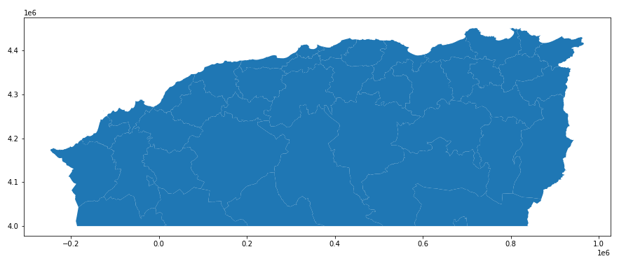
Then clip the rest of the data with the same rectangle (and sorting the values by datetime):
data_gdf = data_gdf.clip(poly).reset_index().drop('index', axis=1).sort_values(['datetime'])
Regional Time Analysis:
We want to first study the variation of fire surface on the whole region in time. This section should be straight forward normal Pandas operations as we won’t need the spatial information.
First, we limit our data to the period of July and August, since the most important fires happened in early August,
july_august_data_gdf = data_gdf.loc[data_gdf.date >= pd.Timestamp('2021-07-01/0000')].loc[data_gdf.date <= pd.Timestamp('2021-08-31/2359')]
Then we do a groupby on the date variable and then sum the areas for each day,
area_sums = july_august_data_gdf.groupby('date').area.sum()
area_sums
date
2021-07-01     93.6030
2021-07-02    114.0144
2021-07-03     45.4706
2021-07-04     39.2529
2021-07-05     45.8119
                ...
2021-08-27     27.7279
2021-08-28     54.5979
2021-08-29    101.9258
2021-08-30    106.9010
2021-08-31     35.1973
Name: area, Length: 62, dtype: float64
Afterwards we will simply plot the Series above:
fig,ax = plt.subplots(figsize=(18,12))

x_ticks = [pd.Timestamp(f"2021-{month}-{day}") for month in range(7,9) for day in range(1,31) if pd.Timestamp(f"2021-{month}-{day}").dayofweek == 4]

ax.plot(area_sums.index, area_sums)
ax.set_ylabel(r'$km^2$', fontsize=12)
ax.set_xlabel('date', fontsize=12)
ax.set_xticks(x_ticks, minor=False)
ax.set_xlim(left=pd.Timestamp('2021-07-01'), right=pd.Timestamp('2021-09-01'))
ax.set_xticklabels([f"  Fri.\n {x.month}-{x.day}" for x in x_ticks])
ax.set_title('Active fire surface in northern Algeria during 2021',fontsize=15)
ax.grid(which='both')

plt.savefig('totaltimeanalysis.png')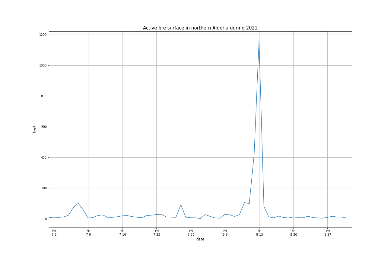
This figure is confirmed by the press. As the worst fires were observed between the 9th of August and the 15th of August. We can also see that there appears to be no correlation between weekdays/weekends(Fridays) and the fires in the months of July and August.
Provincial time analysis:
In this section we’re interested in the time analysis of each province alone to hopefully see the evolution of the fires in the region. Note that due to the nature of the data itself, the studied quantity is not the fire surface but rather the “detected” fires. Since the satellite will only make readings at certain times of the day, and worse due to the size of the country not all pixels are detected at the same time of the day.
Spatial Join:
First, we must find which province does each data point (fire) lie in. To achieve this we use a Spatial Join sjoin, a SQL-like JOIN operation that uses the spatial information between the two GeoDataFrames,
fires_adm_gdf = gpd.sjoin(data_gdf, adm_bnd_north_gdf, how='inner', predicate='within').sort_values('datetime')
fires_adm_gdf.drop(['index_right'], axis=1, inplace=True)
The sjoin function takes the two GeoDataFrames, does an inner JOIN operation where it joins the two GeoDataFrames based on a certain Spatial operation (predicate) which is within in our case.
In other words, it does a JOIN and if the data point from the first GeoDataFrame (the fire) is within the second GeoDataFrame (the province) it joins and adds new columns. The JOIN operation in this case is an inner operation to ensure that each data point is indeed within a province. We also remove the index_right, which corresponds to the indexes from the administrative provinces GeoDataFrame.
Grouping:
Next, we group our fires based on date, time and ADM1_EN (Province). We take the area in each case and sum over it,
grouped_df = fires_adm_gdf.groupby(['date','ACQ_TIME','ADM1_EN']).area.sum()
Plotting the result:
Before we start plotting we’ll need two things: the maximum value for the detected area (w.r.t. date, time and ADM1_EN) for the colorbar value as well as a hash table that links each wilaya (or province) with its index in the adm_bnd_north_gdf GeoDataFrame,
(Also note that we want to further limit the temporal scope to just the second week of August)
max_val = 0
for date in pd.date_range(start='2021-08-08', end='2021-08-15', freq='D'):
    for idx, time_series in grouped_df.loc[date].groupby(level=0):
        for idx2, item in time_series.groupby(level=1):
            if item[0] > max_val:
                max_val = item[0]
max_val
729.5085999999999
ilaya_index = {}
for ind in adm_bnd_north_gdf.index:
    wilaya_index[adm_bnd_north_gdf.loc[ind,'ADM1_EN']] = ind
With that done, we’ll now start the plotting part.
We’ll first create an imgs folder inside our current working directory where we’ll save the frames.
adm_fires = adm_bnd_north_gdf.copy()
adm_fires['area'] = 0
vmin = 0
vmax = max_val
total_series = area_sums.loc[area_sums.index >= pd.Timestamp('2021-07-20/0000')]
for date in pd.date_range(start='2021-08-08', end='2021-08-15', freq='D'):
if date not in grouped_df.index.get_level_values(0):
continue
date_grouped_df = grouped_df.loc[pd.Timestamp(date)]
for time, time_series in date_grouped_df.groupby(level=0):
adm_fires_day = None #Slightly mitigate memory leaks.
adm_fires_day = adm_fires.copy()
for wil, area in time_series.groupby(level=1):
adm_fires_day.at[wilaya_index[wil],'area'] += area[0]
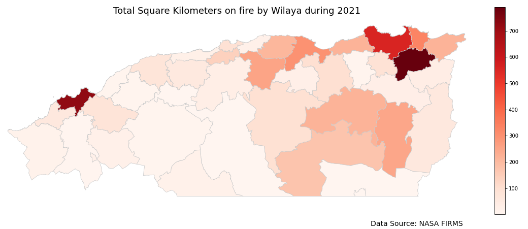
fig,ax = plt.subplots(figsize=(20,15))
adm_fires_day.plot(ax=ax, column='area', cmap='Reds', linewidth=0.8, edgecolor='0.8', vmin=vmin, vmax=vmax, legend=True, legend_kwds={'shrink':0.5, 'pad':0.01, 'fraction':0.1}, norm=plt.Normalize(vmin=vmin, vmax=vmax));
ax.axis('off');
ax.set_title('Detected Square Kilometers on fire by Wilaya', fontsize=15);
ax.annotate(f"{date.date()}/{time}",
xy=(0.1, .225), xycoords='figure fraction',
horizontalalignment='left', verticalalignment='top',
fontsize=10);
#Mini time-series plot
axins = ax.inset_axes([0.05,0.8,0.3,0.2])
current_series = total_series.loc[total_series.index <= pd.Timestamp(f"2021-{date.month}-{date.day}/{time}")]
surface_lim = round(current_series.max())
x_ticks = [date for date in pd.date_range(start='2021-07-25', end=date.date(), freq='D') if date.dayofweek == 4]
axins.plot(current_series.index, current_series)
axins.set_ylabel(r'$km^2$', fontsize=12)
axins.set_xlabel('date', fontsize=12)
axins.set_yticks(range(0,surface_lim+50,50), minor=False)
axins.set_xticks(x_ticks, minor=False)
axins.set_xlim(left=pd.Timestamp('2021-07-20'), right=pd.Timestamp(f"2021-{date.month}-{date.day}"))
axins.set_xticklabels([f" Fri.\n {x.month}-{x.day}" for x in x_ticks])
fig.savefig(f"./imgs/image-{date.day_of_year:03d}-{time}_fires.png", dpi=300);
plt.close(fig)
The first 2 lines creates a copy of the provincial GeoDataFrame/Map and adds a column area to it where we’ll put the total area for each province in each frame. We will copy that copy each time we want to create a new frame.
The total_series fetches data for late July onward for the time sub-plot.
For each date we fetch the data for that date, said data will have time and provincial data within it. Then for each time we create a whole plot. Make sure to name the files in ascending order for ffmpeg.
Then we use ffmpeg to create the gif. To get good colors, we first use ffmpeg to obtain the palette of the images:
ffmpeg -pattern_type glot -i "image-*.png" -vf palettegen palette.png
then we use the palette and the images to generate the gif:
ffmpeg -framerate 2 -pattern_type glot -i "image-*.png" -i palette.png -lavfi paletteuse 2021-wildfires.gif
And the result:
Bonus: Reading HDF-EOS Files:
Before using the FIRMS dataset, I tried to use the scientific data from MODIS. However, there seems to be a misread as the MODIS data only contains “fires” from the Sahara region mostly on rooftops or fires related to oil and gas operations. Reading the HDF files from the MODIS dataset is itself non-trivial, and here I’ll quickly pass over how it can be done.
For reading HDF files, we’ll need GDAL installed as we’ll use the gdal_polygonize.py tool. This data is also not confounded to the borders of the country but are instead just “granules” from the sensors onboard the satellite. Meaning we have to make sure the fires are inside the borders. The data given by the NASA Earth data tool is also split into files, each file for a specific granule and for 8 days at a time. Northern Algeria is within 2 granules, meaning we’ll be getting 2 data files per 8 days. We loop through the files and obtain the date from the file names, use gdal_polygonize.py to obtain a shapefile for the FireMask and MaxFRP SDS’s (Scientific Data Set) within the files, keep the data points within Algeria, then at the end save everything into a GPKG with two layers:
import os
import datetime
import re
import io

import geopandas as gpd
import pandas as pd

file_list = os.listdir('./')

hdf_list = list(filter(lambda x: x[-3:] == 'hdf', file_list))

firemask_gdf = gpd.GeoDataFrame({'DN':[],'geometry':[],'date':[]}, geometry='geometry')
maxfrp_gdf = gpd.GeoDataFrame({'DN':[],'geometry':[],'date':[]}, geometry='geometry')

countries_gdf = gpd.read_file('World_Countries.shp') #World countries shapefile from: https://www.efrainmaps.es/english-version/free-downloads/world/
countries_gdf = countries_gdf.to_crs(3857)
algeria_poly = countries_gdf.loc[3, 'geometry']

cleanshpcom = f"rm polygon*" #Command for cleaning the output of gdal_polygonize once we're done with it.

#Loop through FireMask SDS
for file in hdf_list:
    year = int(re.search(r"MOD14A1.A(\d\d\d\d)(\d\d\d)*", file).group(1))
    days = int(re.search(r"MOD14A1.A(\d\d\d\d)(\d\d\d)*", file).group(2))
    day1 = (datetime.datetime(year,1,1) + datetime.timedelta(days-1)).date()
    for band in range(1,9):
        date = (day1 + datetime.timedelta(band-1))
        days = days + band - 1

        polygonizecom = f"gdal_polygonize.py HDF5:"{file}"://HDFEOS/GRIDS/VNP14A1_Grid/Data_Fields/FireMask polygon.shp geometry"

        os.system(polygonizecom)

        gdf = gpd.read_file('polygon.shp', geometry = 'geometry')

        gdf['date'] = date
        gdf = gdf.loc[gdf.within(algeria_poly)] #Ensure Data points are within Algeria
        firemask_gdf = pd.concat([firemask_gdf, gdf], ignore_index=True)
        os.system(cleanshpcom)

#Loop through MaxFRP SDS
for file in hdf_list:
    year = int(re.search(r"VNP14A1.A(\d\d\d\d)(\d\d\d)*", file).group(1))
    days = int(re.search(r"VNP14A1.A(\d\d\d\d)(\d\d\d)*", file).group(2))
    day1 = (datetime.datetime(year,1,1) + datetime.timedelta(days-1)).date()
    for band in range(1,9):
        date = (day1 + datetime.timedelta(band-1))
        days = days + band - 1

        polygonizecom = f"gdal_polygonize.py HDF5:"{file}"://HDFEOS/GRIDS/VNP14A1_Grid/Data_Fields/MaxFRP polygon.shp geometry"

        os.system(polygonizecom)

        gdf = gpd.read_file('polygon.shp', geometry = 'geometry')

        gdf['date'] = date
        gdf = gdf.loc[gdf.within(algeria_poly)]
        maxfrp_gdf = pd.concat([maxfrp_gdf, gdf], ignore_index=True)
        os.system(cleanshpcom)

firemask_gdf = firemask_gdf.loc[firemask_gdf.DN >= 8]

firemask_gdf.date = firemask_gdf.date.apply(str)
maxfrp_gdf.date = maxfrp_gdf.date.apply(str)

firemask_gdf.loc[firemask_gdf.DN >= 7].to_file('NE_2021.gpkg', layer='FireMask', driver="GPKG")
maxfrp_gdf.to_file('NE_2021.gpkg', layer='MaxFRP', driver="GPKG
All files can be found at: https://github.com/Qfl3x/wildfire-analysis.git